Page 19 - Vol.10

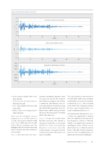
Figure 10. Results after baseline correction

0.5
Acceleration: after baseline correction
0.3
0.1
g
-0.1
-0.3

-0.5
0 10 20 30 40 50 60
second
0.2
Velocity: after baseline correction
0.1

m/s 0

-0.1

-0.2
0 10 20 30 40 50 60
second
0.003
Displacement: after baseline correction
0.002
0.001

m 0
-0.001

-0.002
-0.003
0 10 20 30 40 50 60
second

– Least square straight line fit for domain convolution operates, first The time-domain convolution of
d 0 (t): d 0 +f 0 (t) we copy and inverse the original Ormsby filter with Kaiser window
– C o r r ec t ed d is p l a c e m e n t time history to negative time to have and baseline corrected acceleration
d 1 (t)=d 0 (t)-d 0 -f 0 (t) a symmetric time history, then we is shown in Figure 11, the waveform
– Low – pass Ormsby filter for d 1 (t) start time domain convolution using show there’s low – frequency content
to get d 2 (t) the MATLAB algorithm, but the by low–pass Ormsby filter, it’s
– Final corrected displacement final results will be truncated from easier to understand in Figure 12
d 3 (t)=d 1 (t)-d 2 (t) the point that the peak of Ormsby The final results illustrated in Figure
filter at the time zero.
No w s e t t he O r m sby c or ne r 13 show the amplitude is smaller
frequency fc as 2.8 Hz and ft as Figure 10 shows the results after than the original one because lot of
3.2 Hz, and Kaiser window with baseline correction, the velocity is low frequency content is ‘filtered’
α=10. Figure 8 illustrates the Ormsby integrated from the acceleration which is an important portion of
filter, Kaiser window and the wh ich has been cor rected by earthquake wave, which can be
multiplication of Ormsby filter and base l i ne cor rect ion; a lso the observed in Figure 12 that the portion
Kaiser window, the time window is displacement is integrated from below 3 Hz (the Ormsby frequency
two seconds. corrected velocity. The results are given in this example) plays an
Figure 9 descripts how the time- more reasonable. important role for this earthquake.

NEW FAB TECHNOLOGY JOURNAL JUNE 2013 19