摘要
訊號處理及頻譜分析
Keywords / Seismic Vibration,Signal Processing,Spectral Analysis

The signal processing is the fundamental to deal with digital signal data, such as vibration or earthquake signal. After processing the recorded data, further spectral analysis is needed to identify the features of the signal, and use the feature to carry out such as system identification, vibration source diagnose. This paper introduces the basic signal processing and spectral analysis, and some examples are presented.
Introduction
Both mechanical vibration and seismic vibration are critical to Fab’s operation, thus it is very important to measure and analyze both vibrations. TSMC suffers damages from earthquake in recent years, and there are several cases of vibration impacts on tool operation; that further emphasize the importance of the knowledge on signal processing and spectral analysis. The signal processing knowledge is the basis to understand the parameters for measurement setup and to deal with measured data, it includes Fourier series and Fourier transform, impulse function and generalized function, sampling theory and Nyquist frequency, aliasing, leakage, windowing function, filter design, etc. Most of the topics above are described in the paper “微振量測分析的基礎_數位訊號處理” in 廠務工安季刊第二十二期. So, when relates to corresponding signal processing techniques in this paper, there’ll be just brief statement unless further explanation is needed. Spectral analysis is the knowledge to analyze the recorded data; it includes convolution and correlation theorem, frequency response function (FRF), SI–SO (Single Input–Single Output) and MI–MO (Multi-Input–Multi–output) relationship of linear system, nonlinear system analysis, Z–transform, Hilbert transform, Discrete-time state-space model, Time–domain analysis, system identification, etc. There are so many topics can be discussed, and I will present all these in several parts, trying to let readers fully understand the whole picture.
Type of Signal
Physical phenomena of common interest in engineering are usually measured in terms of an amplitude–versus–time function, referred to as a time history record. There are certain types of physical phenomena where specific time history records of future measurements can be predicted with reasonable accuracy based on one’s knowledge of physics and/or prior observations of experimental results, for example, the force generated by a shaker, the position of a satellite in orbit about the earth, and the response of a structure to a step load. Such phenomena are referred to as deterministic, and methods for analyzing their time history records are well known. Many physical phenomena of engineering interest, however, are not deterministic, that is, each experiment produces a unique time history record which is not likely to be repeated and cannot be accurately predicted in detail. Such data and the physical phenomena they represented are called random.
Classifications of deterministic data
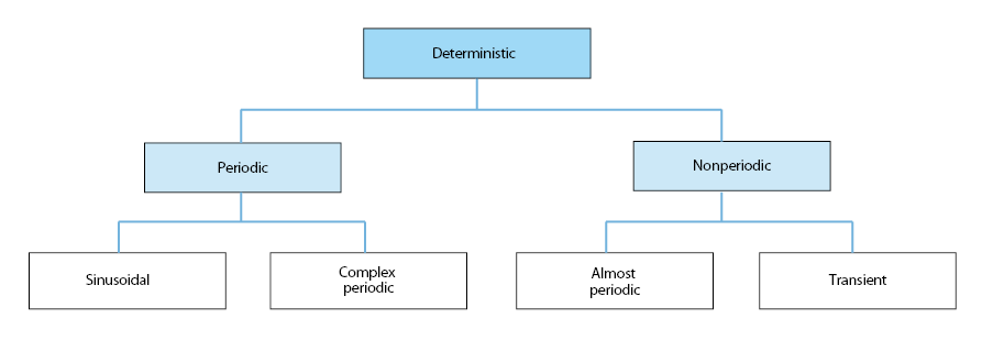
Data representing deterministic phenomena can be categorized as being either periodic or Nonperiodic. Periodic data can be further categorized as being either sinusoidal or complex periodic. Nonperiodic data can be further categorized as being either “almost–periodic” or transient. These various classifications of deterministic data are schematically illustrated in Figure 1. Of course, any combination of these forms may also occur. We will focus on random data, thus these types of deterministic data; will not be discussed in this paper.
Figure 1. Classifications of deterministic data
Classifications of random data
As discuss earlier, data representing a random physical phenomenon cannot be described by an explict mathematical relationship, because each observation of the phenomenon will be unique. In other words, any given observation will represent only one of many possible results that might have occurred.
A single time history representing a random phenomenon is called a sample function (or a sample record when observed over a finite time interval). The collection of all possible sample functions that the random phenomenon might have produced is called a random process or a stochastic process.
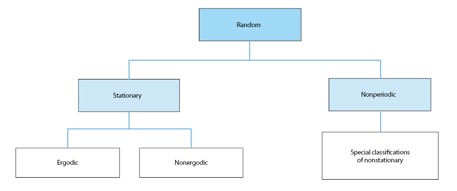
Random processes may be categorized as being either stationary or non-stationary. Stationary random processes may be further categorized as being ergodic or nonergodic. Nonstationary random process may be further categorized in terms of specific types of nonstationary properties. These various classificatins of random processes are schematically illustrated in Figure 2.
Figure 2. Classifications of deterministic data
Analysis of random data
Because no explict mathematical equation can be written for time histories produced by a random phenomenon, statistical procedure must be used to define the descriptive properties of the data. Nevertheless, well-defined input/output relations exist for random data, which are fundamental to a wide range of applications. In such applications, however, an understanding and control of the statistical errors associated with the computed data properties and input/output relationships is essential.
Basic statistical properties of importance for describing single stationary random records are
- Mean and mean square values
- probability density functions
- Autospectral density funstions
μx : mean value, represents the central tendency of stationary record
σx2 : variance, represents the dispersion of stationary record
ψx2 : mean square value, which equals the variance plus the square of the mean, constitutes a measure of the combined central tendency and dispersion.
p(x) : probability density function, represents the rate of change of probability with data value for a stationary record. The function p(x) is generally estimated by computing the probability that the instantaneous value of the single record will be in particular narrow amplitude range centered at various data values, and then dividing by the amplitude range.
Rxx(τ) : autocorrelation function, represents a measure of time-related properties in the data that are seperated by fixed time delays for a atationary record. It can be estimated by delaying the record relative to itself by some fixed time delay τ, then multipling the original record with the delayed record, and averaging the resulting product values over the available record length or over some desired portion of this record length. The procedure is repeated for all time delays of interest.
Gxx(f) : autospectral (also called power spectral) density function, represents the rate of change of mean value with frequency for a stationary record. It is estimated by computing the mean square value in a narrow frequency band at various center frequencies, and then dividing by the frequency band. The total area under the autospectral density function over all frequencies will be the total mean square value of the record. The partial area under the autospectral density from f1 to f2 represents the mean square value of the record associated with that frequency range.
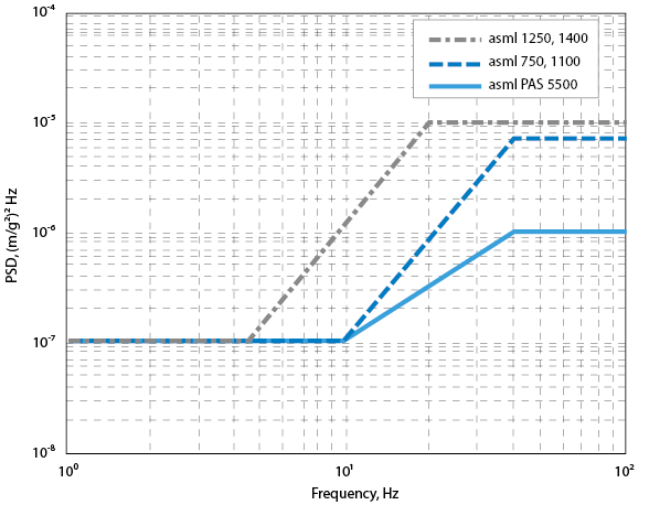
The vibration specification of ASML scanner is presented by autospectral density of acceleration, as illustrated in Figure 3.
Figure 3. Vibration specification of scanner
Convolution
Convolution of two functions is a significant physical concept in many diverse scientific fields. However, as in the case of many important mathematical relationships, the convolution does not readily unveil itself as to its true implications. To be more specific, the convolution integral is given by
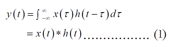
Function y(t) is said to be the convolution of the functions x(t) and h(t). Note that it is extremely difficult to visualize the mathematical operation of Equation (1), the graphical interpretation please refer to “微振量測分析的基礎_數位訊號處理” in 廠務工安季刊.
Time-convolution theorem
Possibly the most important and powerful modern scientific analysis is the relationship between Equation (1) and its Fourier transform. This relationship, known as time-convolution theorem, allows one the complete freedom to convolve mathematically (or visually) in the time domain by a simple multiplication in the frequency domain. That is, if h(t) and x(t) have the Fourier transform H(f)and X(f) respectively, then h(t)*x(t) has the Fourier transform H(f)X(f). In other words, the Fourier transform of the convolution of two functions in time domain is equal to the multiplication of their Fourier transform in frequency domain. (Note that the operator “*” means convolution operation)
Frequency-convolution theorem
Similar to the time-convolution theorem, we can equivalently go from convolution in the frequency domain to multiplication in the time domain by using the frequency-convolution theorem: the Fourier transform of the product h(t)x(t) is equal to the convolution H(f)*X(f)
Ormsby Filter
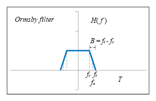
To reduce the error in the filtering effects, a numerical filter developed by J. F. Ormsby is currently implemented in the programs for processing seismic data in this study. Figure 6 shows the parameters defining the transfer function of the Ormsby filter.
Figure 6. Illustration of Ormsby filter design
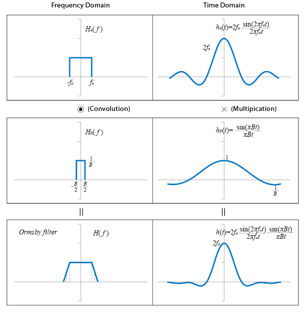
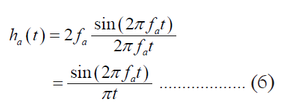
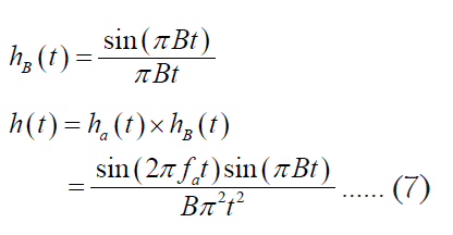
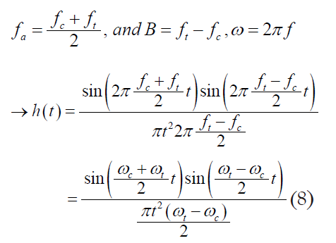
They are the cut-off and roll-off termination frequencies (fc and ft), and the transition bandwidth, B. The transfer function of Ormsby filter is the convolution of that of a sinc filter with cut-off frequency fa and a rectangular function of base B and unit area. The resulting weighting function for this filter is
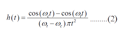
where ωc=2πfc and ωt=2πft. The effect of the transition zone is to attenuate the weighting function of the sinc filter with cut-off frequency fa. The filtering process can be described as a convolution of the original signal y(t) with the filter h(t); therefore,
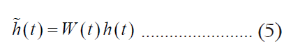
From Equation (3) the implication of using a finite number of terms for the numerical convolution is necessary. To reduce the leakage effect, the Kaiser window W(t) is used.
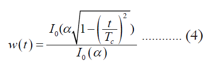
Where Tc is the cut-off time, and α is the parameter controlling the shape of the window. I0(α) represents the modified zeroth order Bessel function. The truncated filtering function  , is given by
Recall the Fourier transform pair of rectangular signal is a sinc function as Figure 4.
Figure 4. Sinc function and its Fourier transform
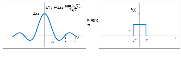
Figure 5. Ormsby filter
Using the symmetry property of Fourier transform:

where F means Fourier transform
The frequency domain convolution of Ha(f) and HB(f) is equal to the multiplication of ha(t) and hB(t) in time domain. We can get the equivalent time domain function ha(t) and hB(t) by the symmetry property of Fourier transform.
Since all the functions are even function, thus is very easy to get the equivalent time domain function by replace variable f as t. The graphical illustration is as Figure 7.
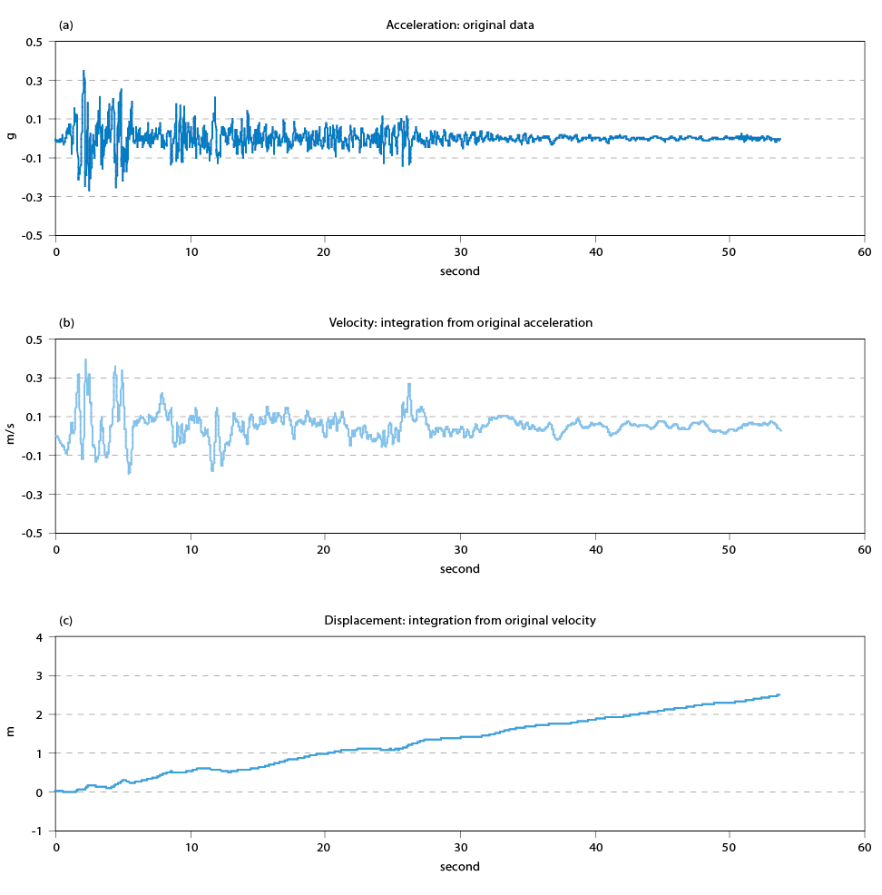
Figure 7. (a) Original earthquake acceleration time history; (b) Velocity time history without any baseline correction; (c) Displacement time history without any baseline correction
by the relationship :
Application on Seismic Time History Analysis
The seismic data are always recorded in acceleration unit, but the velocity and displacement are also the important parameters for analysis, thus we have to integrate the acceleration time history to get velocity time history; and integrate again to get displacement time history. But if the acceleration time history has a shift to zero mean (either constant or inclined) then the integration will amplify this shift, thereby causes the velocity and displacement time history into incorrect results. Figure 8 illustrates the velocity and displacement time history integrated from acceleration time history without any baseline correction.
Figure 8. Ormsby Low-pass filter and Kaiser window (with alpha=10)
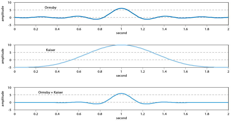
Figure 7c shows the maximum displacement is over 2 meters, it’s obviously impossible, thus the baseline correction procedures are needed, and the procedures are
- For recorded acceleration a(t), least square fit straight line: a0+c0(t)
- Corrected acceleration a1(t)=a(t)-a0-c0(t)
- Low-pass Ormsby filter for a1(t) to get a2(t)
- Final corrected acceleration a3(t)=a1(t)-a2(t)
- Integrate a3(t), assume v(0)=0 (zero initial velocity), get v0(t)
- Least square straight line fit for v0(t): v0+e0(t)
- Corrected velocity v1(t)=v0(t)-v0-e0(t)
- Low-pass Ormsby filter for v1(t) to get v2(t)
- Final corrected velocity v3(t)=v1(t)-v2(t)
- Integrate v3(t), assume d(0)=0 (zero initial displacement), get d0(t)
- Least square straight line fit for d0(t): d0+f0(t)
- Corrected displacement d1(t)=d0(t)-d0-f0(t)
- Low–pass Ormsby filter for d1(t) to get d2(t)
- Final corrected displacement d3(t)=d1(t)-d2(t)
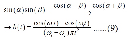
Now set the Ormsby corner frequency fc as 2.8 Hz and ft as 3.2 Hz, and Kaiser window with α=10. Figure 8 illustrates the Ormsby filter, Kaiser window and the multiplication of Ormsby filter and Kaiser window, the time window is two seconds.
Figure 9 descripts how the time-domain convolution operates, first we copy and inverse the original time history to negative time to have a symmetric time history, then we start time domain convolution using the MATLAB algorithm, but the final results will be truncated from the point that the peak of Ormsby filter at the time zero.
Figure 9. Convolution description
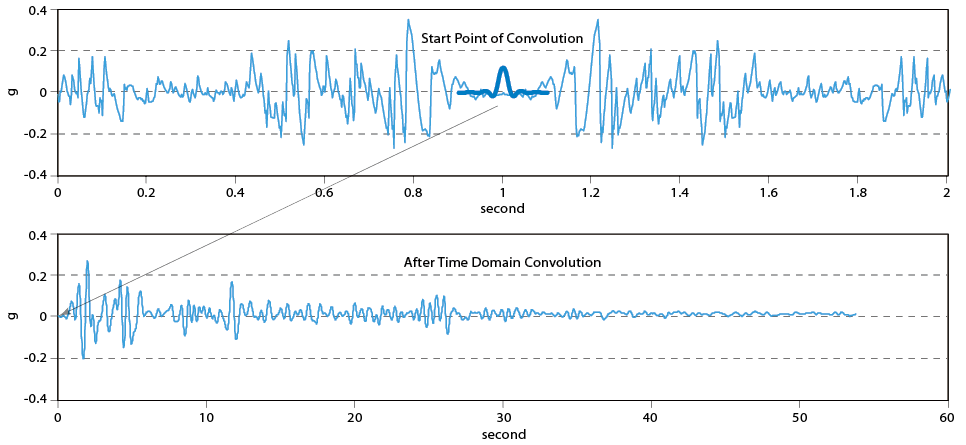
Figure 10 shows the results after baseline correction, the velocity is integrated from the acceleration which has been corrected by baseline correction; also the displacement is integrated from corrected velocity. The results are more reasonable.
Figure 10. Results after baseline correction
The time-domain convolution of Ormsby filter with Kaiser window and baseline corrected acceleration is shown in Figure 11, the waveform show there’s low–frequency content by low–pass Ormsby filter, it’s easier to understand in Figure 12
Figure 11. Results after Ormsby filter + Kaiser window
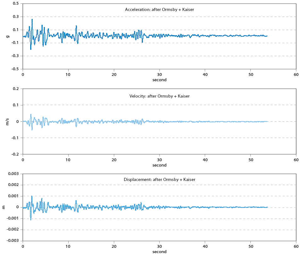
Figure 12. Fourier Spectrum of different stage
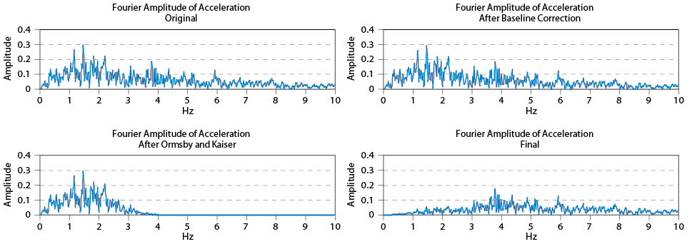
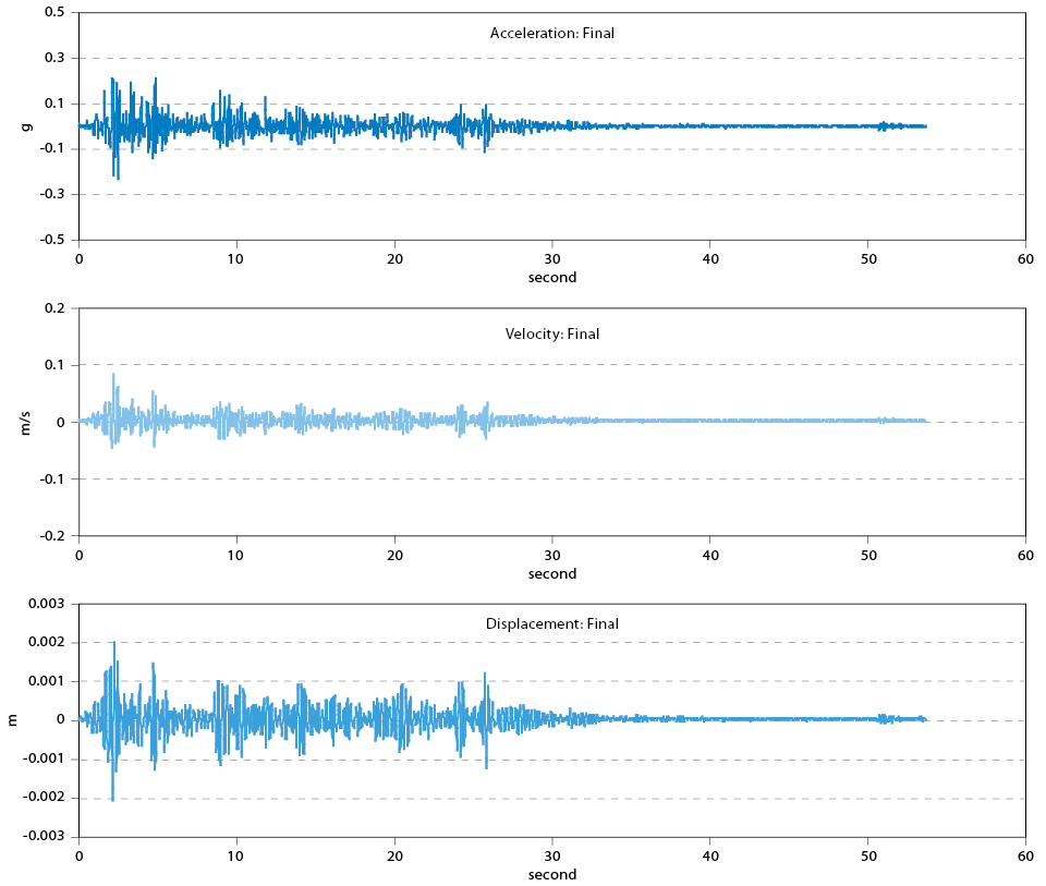
The final results illustrated in Figure 13 show the amplitude is smaller than the original one because lot of low frequency content is ‘filtered’ which is an important portion of earthquake wave, which can be observed in Figure 12 that the portion below 3 Hz (the Ormsby frequency given in this example) plays an important role for this earthquake.
Figure 13. Final Results
Conclusion
This paper introduces the basic concept of signal type, analysis of random type, and possibly the most important convolution theorem, the widely used and fundamental procedure to deal with earthquake time history data, there are still many applications to be presented, they will be presented in the succeeding papers.
參考文獻
- A. Papoulis, The Fourier Integral and Its Application, second edition, New York: McGraw-Hill, 1986.
- Andre Preumont, Random Vibration and Spectral Analysis, Kluwer Academic Publishers, 1994.
- Alan V. Oppenheim, Ronald W. Schafer & John R. Buck, Discrete-Time Signal Processing, second edition, Prentice-Hall Inc. 1999.
- Boaz Porat, A Course in Digital Signal Processing, John Wiley & Sons, Inc. 1997.
- D.E. Newland, An Introduction to Random Vibrations, Spectral and Wavelet Analysis, third edition, Longman Inc., 1993.
- E. Oran Brigham, The Fast Fourier Transform and its Applications, Prentice-Hall, 1988.
- Julius S. Bendat& Allan G. Piersol, Engineering Applications of Correlation and Spectral Analysis, second edition, John Wiley & Sons, Inc. 1993.
- Julius S. Bendat& Allan G. Piersol, Random Data-Analysis and Measurement Procedures, third edition, John Wiley & Sons, Inc. 2000.
- Kennth G. McConnell, Vibration Testing-Theory and Practice, John Wiley & Sons, Inc. 1995.
- Paolo L. Gatti and Vittorio Ferrari, Applied Structural and Mechanical Vibrations, Theory, Methods and Measuring Instrumentation, E & FN SPON, 1999.
- Steven L. Kramer, Geotechnical Earthquake Engineering, Prentice-Hall, 1996
- Vinay K. Ingle & John G. Proakis,Digital Signal Processing Using MATLAB, Brooks/Cole Publishing Company, 2000.
- W.T. Thomson & M.D. Dahleh, Theory of Vibration with Applications, fifth edition, Prentice-Hall, 1998.
- S. Gade& H. Herlufsen, Use of Weighting Functions in DFT/FFT Analysis (Part II), Technical Review, Nos. 3 and 4, 1987, Bruel&Kjaer.
留言(0)